DroneMapper Labs: geoBit Ground Control Point Target Systems
Jon-Pierre Stoermer, CTO – DroneMapper.com
Jon-Pierre Stoermer, CTO – DroneMapper.com
geoBits.io
We often get requests from our customers to develop additional value-added features and algorithms to extract more meaningful information from aerial or terrestrial data collections. Recently, the area of Precision Agriculture has seen enormous growth triggered by reduced technology costs and overall interest in new/emerging technologies. The integration of UAS systems, GPS, RTK and other geo-spatial technologies into the farming sector allows a whole new world of opportunities. Although technology can't solve all of our tasks, it can certainly help in new and exciting ways!
A common task for an Agronomist is the creation of management zones or "area's of interest" based on the available data. The data could be an aerial imagery collection in NIR, yield data from a terrestrial collection, EC soil samples, or a combination of all. Historically, a large amount of research has been devoted to automating the process of extracting appropriate zones when high resolution spatial data is available. This can also be a complicated and time consuming task.
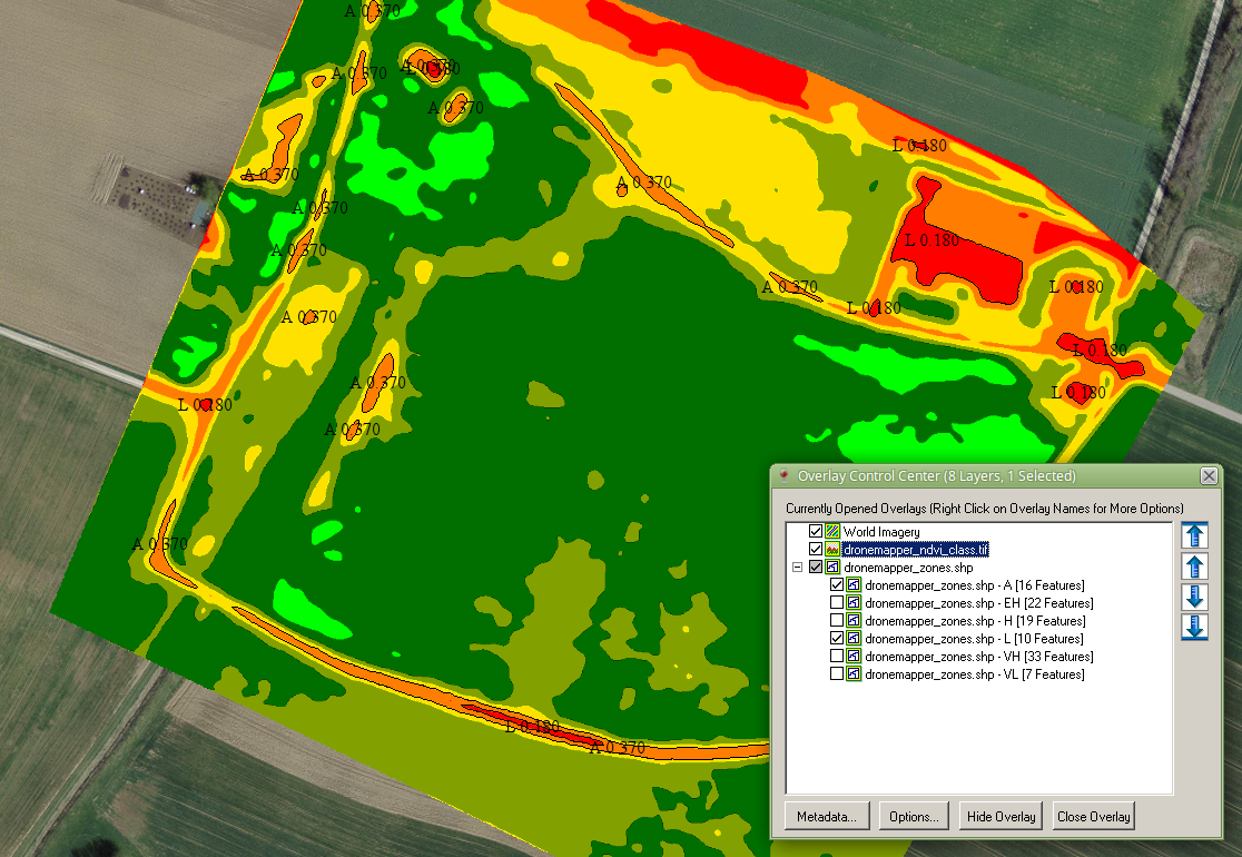
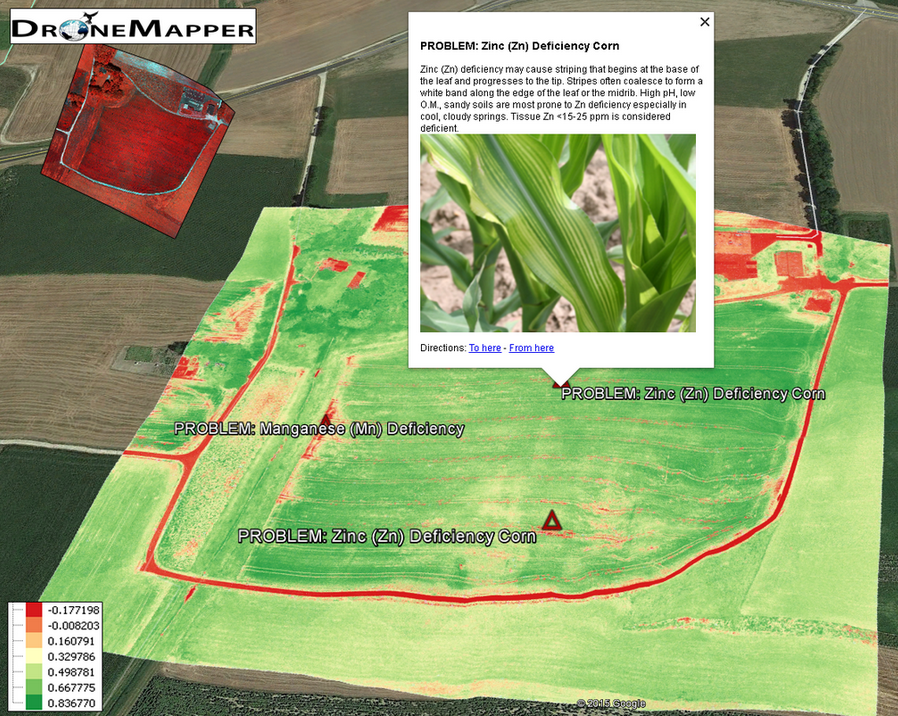
"Normalized difference vegetation index (NDVI) are closely related to many vegetation parameters such as leaf area index, vegetation cover, vegetation biomass and crop growth, so is often used to monitor crop growth and predict crop yield." [1]
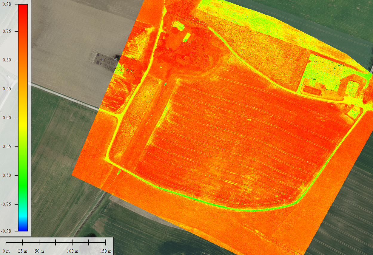
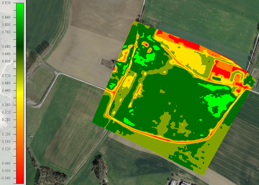
The image above shows a classified NDVI GeoTIFF where each pixel falls into one of the following categories:
Once classification is completed, DroneMapper generates a shapefile with management zones. The shapefile output is UTM WGS84 format and compatiable with major agriculture software providers such as SST, SMS, Apex, etc.
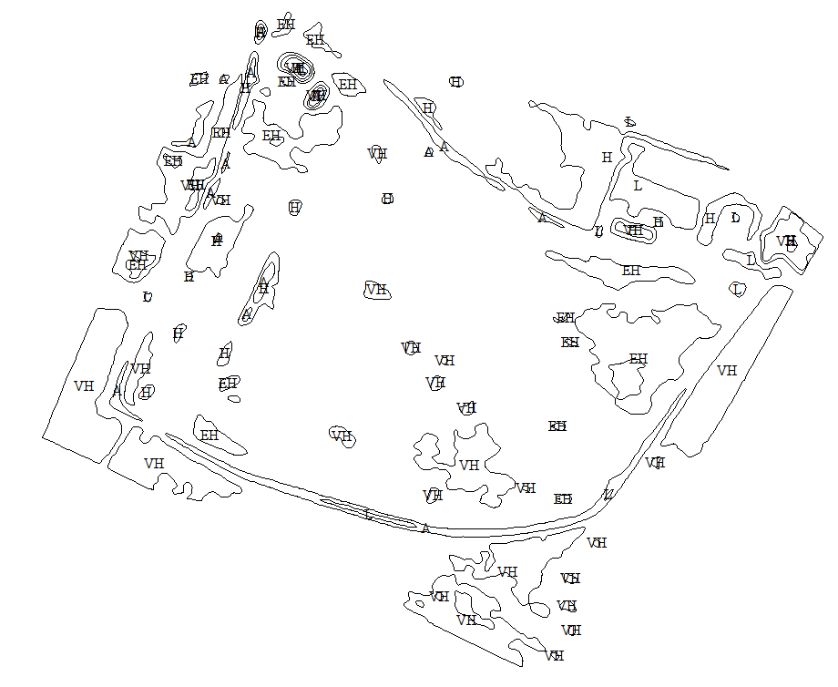
Each polygon in the generated shapefile includes records in the .dbf file with the following information:
This allows sorting or grouping of the polygons based on .dbf column values.
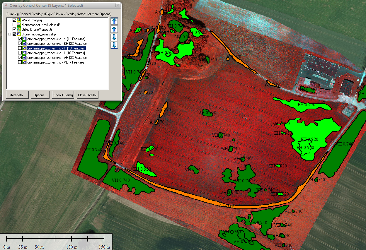
The algorithm completes processing after a few minutes and could easily be adapted to provide point data for Crop Scouting locations, ground truthing, etc.
Download the data generated in this post here or on our samples page. For more information on agriculture management zones we recommend the following link. Please let us know if you have any questions!
Here is a simplified Excel spreadsheet that can be used to assist UAS aerial photo mission planning for those that don’t have access to mission planning software either provided with the UAS or custom written. The spreadsheet uses the following inputs (cells are highlighted in yellow) provided by you for your mission:
After you have input the various parameters for your mission the spreadsheet provides the following outputs (these cells have no color fill and should be locked to the user):
Suggestions:
Pierre Stoermer, CEO – DroneMapper.com
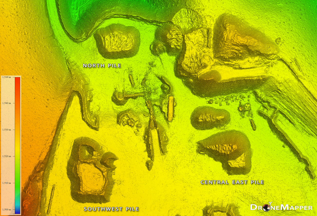
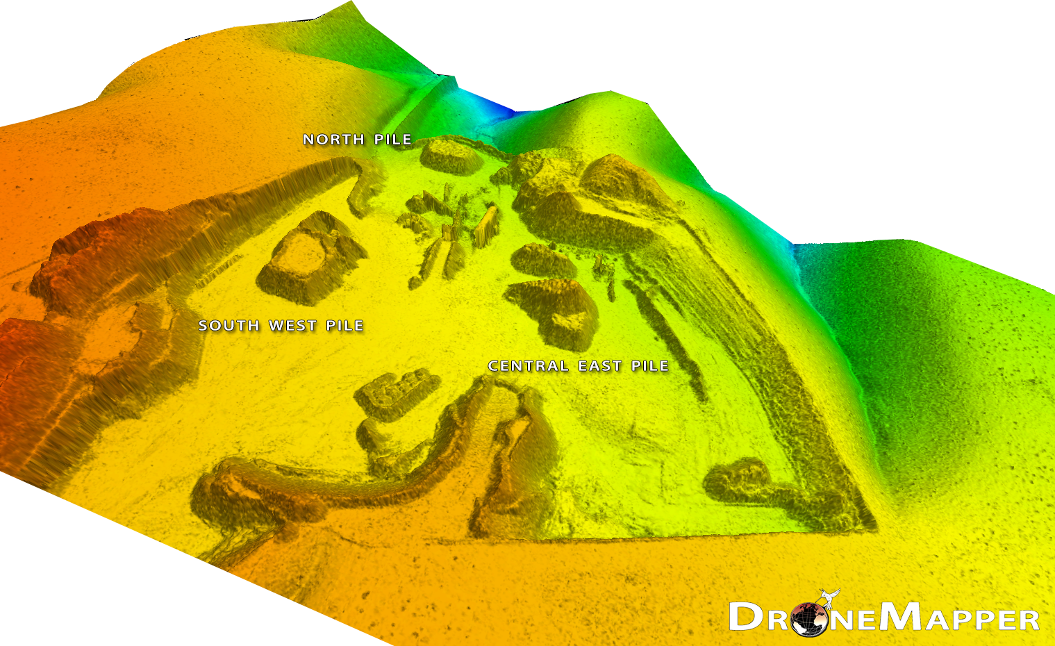
We utilized Globalmapper (GM), version 16.1, to determine stockpile volumes for the BLM gravel pit example. A Canon SX 260 HS was used to collect 240 images at a ground sample distance of 3.2 cm. Dronemapper processed the imagery generating the geo-referenced orthomosaic and DEM for the scene. For this analysis we imported the DEM into GM and performed volumetric estimation of three stockpiles. The three piles are identified in the DEM image below.
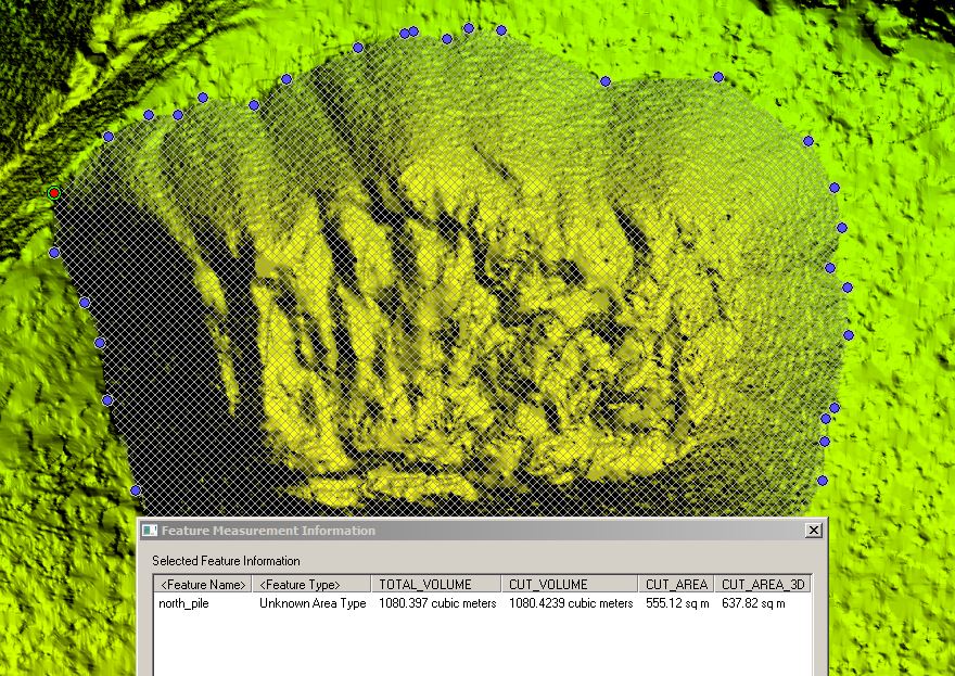
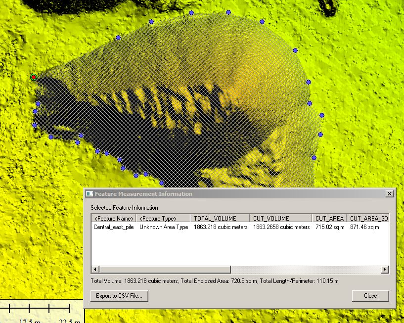
After importing the DEM the digitizer tool was used to generate an area at the base of each of the stockpiles. Once the pile areas were defined we applied elevations from the terrain to each of the three pile areas. We then computed pile volumes. GM generates a flattened terrain surface (reference) beneath the pile and a pile surface. The difference between these two 3-D surfaces computes the volume of the pile. The table outlines the measurements made on each pile.
| Pile Name | Total Volume (m3) | Cut Volume (m3) | Cut Area (m2) | Cut Area 3-D (m2) |
| North Pile | 1080.397 | 1080.424 | 555.12 | 637.82 |
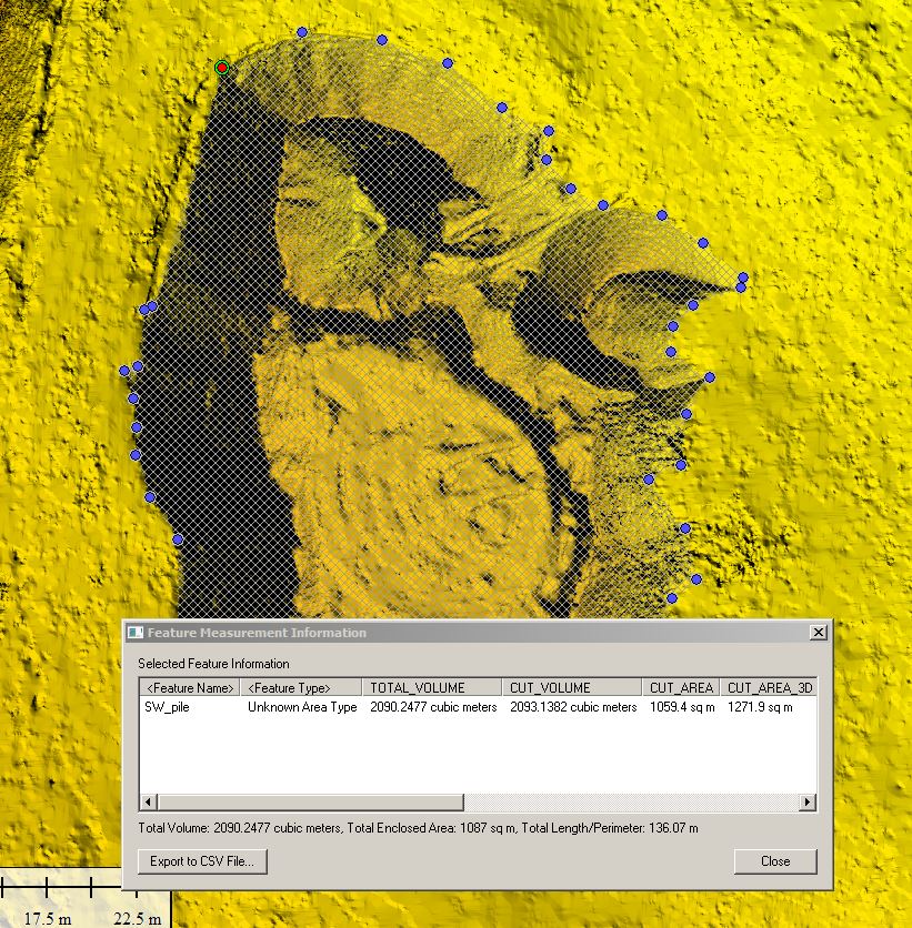
| South West Pile | 2090.248 | 2093.138 | 1059.4 | 1271.9 |
| Central East Pile | 1863.218 | 1863.266 | 715.02 | 871.46 |
The three measurements are illustrated in the next three screenshots. The last screenshot shows a 3-D view of the identified piles that were measured to give the viewer perception of their relative sizes. Besides cut volumes, GM also performs fill volumes, valuable for the mining and construction industries.
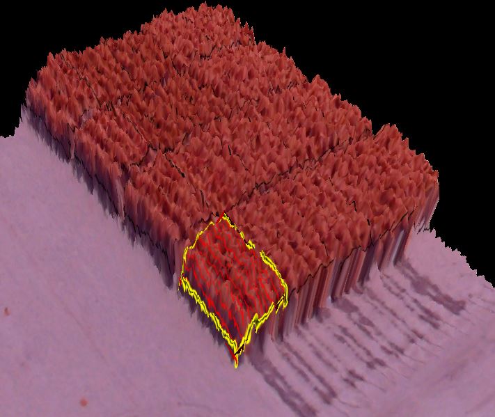
This same technique can be used for estimating above ground biomass for crops. A section of a 3-D model of a research corn field is illustrated below. Imagery was collected at 5 cm GSD in the NIR. One of the plots within the field is identified with a plot shapefile (in yellow). The average plot height was estimated at 216 cm using the volume and area generated by GM. In this case we could not utilize two 3-D surfaces to compute the volume since adjacent plots obscured the terrain below the plot of interest. Instead, we used a fixed mean elevation of the terrain as the reference to compute the volume of the plot’s 3-D surface.
We will be working with precision agricultural specialists this growing season to track a set of crops/fields on a weekly basis. The DEM will be generated for each imagery collection of the crop through the growing season. Biomass volume estimation will be computed for each collection for all of the plots in the field. Plot biomass accumulation will be tracked weekly, statistically analyzed and correlated with plant genetics, field treatments and other phenomenology collections. We hope to report on this by the end of this year – so stay tuned!